Point-of-View Invariance and Noether’s Theorem

Noether’s theorem is an important theorem that relates invariance of space-time transformations to the laws of conservation: space-translation invariance to the conservation of linear momentum, space-rotation invariance to the conservation of angular momentum, and time-translation invariance to the conservation of energy. The models of physics are point-of-view invariant: physical models cannot depend on any particular position in space or moment in time.

A video version of this episode showing the equations is available on YouTube.

Where do the laws of physics come from? This question is the subtitle of Victor Stenger’s 2006 book Comprehensible Cosmos. I think this question is one version of the more general guiding question of my whole intellectual life: why are things the way they are? Stenger has a very interesting response to this question, which is based on what he calls principle of point-of-view invariance “The models of physics cannot depend on any particular point of view.”

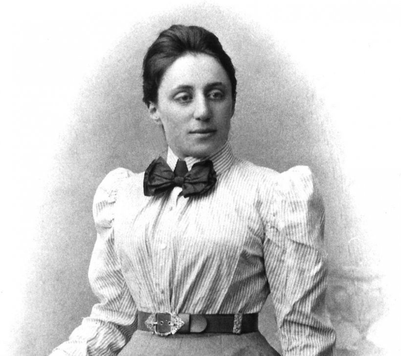
The path from this principle to the laws of physics goes through an important theorem known as Noether’s Theorem. This theorem was developed by Emmy Noether in 1918. Put briefly, the theorem says that symmetries in a system generate conserved quantities. Anyone who’s studied (and remembers) physics will know of the conservation of momentum, conservation of angular momentum, and the conservation of energy. These conservation laws are absolutely foundational. And what’s remarkable is that there’s a reason for them. These conservation laws come from symmetries. The conservation of momentum, angular momentum, and energy come from symmetries of translation, rotation, and time.

Stenger puts it this way: “In any space-time model possessing time-translation invariance, energy must be conserved. In any space-time model possessing space-translation invariance, linear momentum must be conserved. In any space-time model possessing space-rotation invariance, angular momentum must be conserved. Thus, the conservation principles follow from point-of-view invariance. If you wish to build a model using space and time as a framework, and you formulate that model so as to be space-time symmetric, then that model will automatically contain what are usually regarded as the three most important ‘laws’ of physics, the three conservation principles.”

To me this is quite remarkable. But maybe I’m just easily impressed. So I went online to see how others view all this. I looked up on Quora responses to the question: “What is the significance of Noether’s theorem?” Here are some of the responses:

“I think it is almost the thing that makes sense of physics. Physics is based on a large number of conservation rules – conservation of energy, momentum etc. Without Noether’s Theorem, all you can say is that they are conserved – they are just givens. With the Theorem, you can say that they arise from the symmetries of the space we live in. [In] a space which did not have these symmetries… these conservations would be so different from the space we know as to be unrecognizable. It derives the otherwise arbitrary conservation rules from intuitively understood symmetries. Brilliant.” (Alec Cawley)

“Most of fundamental physics could be interpreted as positing a symmetry, then handing that symmetry off to Ms. Noether and asking her to tell us what the resulting physics is. In other words, without Noether’s Theorem, there wouldn’t be most of modern physics.” (Brent Follin, PhD in Theoretical Cosmology)

And my favorite.

“It’s a matter of life and death! Being a Physics student, the Noether’s theorem is extremely important with everything I do. If it were falsified, the whole structure of modern physics would crumble!” (Abhijeet Borkar, PhD in Physics (Astrophysics))

So it’s a pretty big deal. Hopefully that sparks some interest. Now let’s dig into it and see how it works.

Invariance and Transformations

First, let’s revisit this idea of point-of-view invariance. One of the first things you do in a physics problem is define your coordinates. If you’re on the surface of the Earth you usually set one axis pointing up from the center of the Earth. This is what we’re used to thinking of as “up”. That’s because in our everyday experience there pragmatically is an obvious coordinate system to use. There’s an up and a down. But that’s because we reference our everyday experience relative to Earth, which we’re living on. But we know, at least since the Copernican revolution, that this coordinate system isn’t absolute. The Earth isn’t the center of the universe, even if it is the center of our lived experience. But it’s not just that. There is no center of the universe at all. There’s no absolute up or down.

That doesn’t mean that we don’t use coordinates. Of course we do. We have to. But it does mean that the coordinate system we use is not absolute. We’ll usually use one that makes things easy for our calculations. But the system we represent in one coordinate system can also be represented in a different coordinate system.

This is easy to see with vectors. Let’s represent a vector on an x-y Cartesian coordinate system. The vector will start from the origin (0,0) and go out to point (4,3). What’s the magnitude of this vector? We calculate that by the equation:

√((x2 – x1)^2 + (y2 – y1)^2)

And plugging in our  values:

√((4 – 0)^2 + (3 – 0)^2) = √((4)^2 + (3)^2) = √(16+ 9) = √(25) = 5

The magnitude of this vector is 5.

Now let’s change the coordinate system shifting it 2 to the right and 7 up. Now this same vector starts at (-2,-7) and goes out to (2,-4). What’s the magnitude?

√((-2 – 2)^2 + (-7 – -4)^2) = √((-4)^2 + (3)^2) = √(16+ 9) = √(25) = 5

The magnitude is still 5.

Now let’s go back to the first coordinate system and rotate it 30 degrees counter-clockwise. 30 degrees in radians is π/6 radians. We make this transformation using the rotation matrix

R = [[cos θ,-sin θ], [sin θ, cos θ]]

And multiply R by our vector [[x],[y]].

The result is

Rv = [[x cos θ – y sin θ], [x sin θ + y cos θ]]

Rv = [[3/2 * √(3) – 2], [3/2 * 2 x √(3)]]

Rv = [0.598], [4.964]]

For our transformation θ is π/6 radians. Our new vector coordinates are (0,0) and approximately (0.598,4.964). Now the moment of truth, after all of that. What’s the magnitude? It’s

√((0.598- 0)^2 + (4.964 – 0)^2) = √((0.598)^2 + (4.964)^2) = √(0.358 + 24.642) = √(25) = 5

The magnitude is still 5.

When we look at this visually, it’s actually not surprising. The vector stays the same in all these cases. It’s just the coordinate system that’s moving around. This is the basic idea of invariance. And I think it gives a general sense about how something can remain constant if it doesn’t depend on these coordinate system transformations.

The Lagrangian

Before getting to Noether’s Theorem itself, we need to talk about the Lagrangian because Noether’s Theorem is expressed in terms of it. The Lagrangian is a function that describes the state of a system and is equal to the difference between the total kinetic energy, T, and the total potential energy, V, of a system.

L = T – V

The Lagrangian is used in Lagrangian mechanics and is a different way of looking at systems than Newtonian mechanics. Instead of looking at forces, as in Newtonian mechanics, in Lagrangian mechanics we’re looking at energies. The Lagrangian is a function of spatial coordinates and their derivatives with respect to time. Spatial coordinates could be the familiar Cartesian x,y,z coordinates but it’s customary to generalize these with a single variable. For example, q. For multiple spatial coordinates we can just number them off, q = {q1, q2,…, qn]. The time derivative of q is,. The time derivative of a spatial coordinate is velocity.

So some of the familiar quantities from Newtonian mechanics will be expressed differently in Lagrangian mechanics. Most notably, momentum. In Newtonian mechanics we express momentum as mass times velocity.

p = mv

To express this in terms of a Lagrangian let’s change v to . So,

p = mq̇

Now the Lagrangian is the difference between kinetic energy and potential energy.

L = T – V

Kinetic energy is

T = 1/2 mv^2

Or

T = 1/2 m q̇^2

So we can rewrite the Lagrangian as

L = 1/2 mq̇^2 – V

Now taking the derivative with respect to

δL/δq̇ = mq̇

And mq̇ = p, so

p = δL/δq̇

And that’s the equation for momentum in terms of the Lagrangian.

p = δL/δq̇

So momentum is the derivative of the Lagrangian with respect to velocity. Also the derivative of the kinetic energy with respect to velocity.

The Hamiltonian

Another function I want to go over before moving on to Noether, and that’s the Hamiltonian function. The Hamiltonian is similar to the Lagrangian, except that it’s the sum of kinetic energy and potential instead of the difference between them.

H = T + V

The Hamiltonian is the total energy of the system. And we can express this in terms of the Lagrangian. Since L = T – V we can express the potential energy as

V = T – L

Substituting this into the Hamiltonian

H = T + V

H = T + (T – L)

H = 2T – L

H = 2(1/2 mq̇^2) – L

H = (mq̇)q̇ – L

Since p = mq̇

H = pq̇ – L

And since also p = δL/δq̇

H = (δL/δq̇)q̇ – L

This is the expression for the total energy in terms of the Lagrangian.

H = (δL/δq̇)q̇ – L

The Lagrange-Euler Equation of Motion

One more equation we should introduce before getting into Noether’s theorem is the Lagrange-Euler equation, also called the equation of motion. This has the form

d/dt (δL/δq̇) = δL/δq

What is this equation saying? Let’s translate this out of the Lagrangian form into the more familiar Newtonian quantities. An equivalent form of this equation is:

dp/dt = -δV/δq = F

d(mv)/dt = F

ma = F

This is Newton’s second law. It’s just expressed in a different form with the Lagrangian, which again is:

d/dt (δL/δq̇) = δL/δq

We’ll be plugging this equation into a lot of things in the foregoing so it’s important.

Noether’s Theorem

Now, let’s move to Noether’s theorem. We’ll look at Noether’s theorem for the conservation of momentum, the conservation of angular momentum, and for the conservation of energy.

We start with the Lagrangian as a function of position, q, and velocity, .

L(q, q̇)

What we’re going to do is apply the following transformation on q and .

q q(s)

q̇(s)

If our Lagrangian has symmetry it should not change under this transformation to s. Expressed mathematically this means

d/ds L(q(s), q̇(s)) = 0

Let’s propose that under this transformation that there is a conserved quantity, C, of the following form:

C = (δL/δq̇)(δq/δs)

And since it is a conserved quantity it does not change over time. That is

dC/dt = 0

And here’s the proof for that. Take the proposed conserved quantity C and take the time derivative of it.

C = (δL/δq̇)(δq/δs)

dC/dt = d/dt ((δL/δq̇)(δq/δs))

Since we have two variables, q and , we need to apply the product rule:

dC/dt = d/dt (δL/δq̇) * (δq/δs) + (δL/δq̇) * (δq̇/δs)

Now, recall the Euler-Lagrange equation of motion.

d/dt (δL/δq̇) = δL/δq

We’re going to plug that in here to get.

dC/dt = (δL/δq)(δq/δs) + (δL/δq̇)(δq̇/δs)

What do we have here? The right hand side of this equation is what we get when we apply the chain rule to the derivative of the Lagrangian with respect to s.

d/ds L(q(s), q̇(s)) = (δL/δq)(δq/δs) + (δL/δq̇)(δq̇/δs)

And this is equal to 0. So

dC/dt = (δL/δq)(δq/δs) + (δL/δq̇)(δq̇/δs) = d/ds L(q(s), q̇(s)) = 0

And

dC/dt = 0

So what’s been proved here is that if the Lagrangian, L, does not change with respect to transformation, s, than the conserved quantity, C, doesn’t either.

That’s Noether’s Theorem. Now let’s look at some applications, examples of conserved quantities that result from different symmetries.

Conservation of Linear Momentum

To get the conservation of linear momentum we’re going to say that the Lagrangian is symmetric under continuous translations in space. Our spatial coordinates are

q = {q1, q2,…, qn].

And we’ll apply the transformation

q q(s)

where

q(s) = q + s

So we’re just sliding our coordinate system over by an interval, s.

The conserved quantity C is

C = (δL/δq̇)(δq/δs)

Taking the derivative of q with respect to s

δq/δs = δ/δs (q + s) = 1

So C becomes

C = (δL/δq̇) = p

Which is momentum. So when we apply the spatial transformation

q à q(s)

The conserved quantity, C, is momentum, p. In other words, the conservation of momentum results from symmetry in space. To give some interpretation, this means that the system has no dependence on where it is in space. It’s not being acted upon by any external forces. If there were an external force then it would depend on it’s location in space.

Recall that force is equal to

F = ma

F = m(dv/dt)

F = d/dt (mv)

F = dp/dt

Force is equal to the rate of change in momentum with respect to time. So clearly if there is a non-zero external force acting on the system momentum is not constant.

If there is an applied force external to the system, like with a spring, then momentum is obviously not conserved. And with such forces location makes a difference. With a spring it matters how much the spring is stretched. So momentum is not conserved in such cases where there’s not symmetry in space for that system. But in systems that do have symmetry in space, momentum is conserved.

Conservation of Angular Momentum

To get the conservation of angular momentum we’re going to say that the Lagrangian is symmetric under continuous rotations in space.

We apply the transformation.

q q(s)

In which case s is some angle of rotation. This is a two-dimensional case where q is represented by the matrix

[[q1],[q2]]

We make this transformation using the rotation matrix

R = [[cos s,-sin s], [sin s, cos s]]

And multiply R by our matrix [[q1],[q2]]

The result is

Rq = [[cos s,-sin s], [sin s, cos s]] * [[q1],[q2]]

For very small values of s near 0

sin(s) ≈ s

cos(s) ≈ 1

That’s from Taylor’s series expansion to the first order. This makes the rotation matrix is equal to

[[1, -s], [s, 1]]

So the transformation is

[[1, -s], [s, 1]] * [[q1],[q2]]

The result of this transformation is that

q1 → q1 – s * q2

q2 → q2 + s * q1

For reasons that will be clear shortly, let’s differentiate these.

dq1/ds = -q2

dq2/ds = q1

Now let’s bring in our conserved quantity, C

C = (δL/δq̇)(δq/δs)

And since

q = {q1,q1}

C = (δL/δq̇1)(δq1/δs) + (δL/δq̇2)(δq2/δs)

Or in terms of momentum, p

C = p1 * (δq1/δs) + p2 * (δq2/δs)

The derivatives in this equation are equal to the derivatives we just calculated for q1(s) and q2(s). So, plugging those in:

C = q1 * p2 – q2 * p1

And this is equal to the cross product

C = q x p

Which is angular momentum L. Angular momentum is equal to the cross product of linear momentum and the position vector. So

C = L

The conserved quantity, C, is angular momentum, L. In other words angular momentum results from symmetry of rotation. To give some interpretation again, this is the condition in which the system has no external rotational forces, i.e. torque. To use the example of a spring again, if this were a system where we’re winding up a torsion spring then angular position very much matters. The tighter we wind it up the higher the torque. In that kind of system angular momentum is not conserved. But in the absence of that kind of torque, angular position and rotation don’t matter. So angular momentum is conserved.

Conservation of Energy

To get the conservation of energy we’re going to say that the Lagrangian is symmetric in time. So we have our Lagrangian

L(q, q̇)

And we’re going to say that it doesn’t change with time

dL/dt = 0

Let’s see what follows from this. First let’s to the derivative of the Lagrangian with respect to time. To do this we apply the chain rule.

dL/dt = (δL/δq)(δq/δt) + (δL/δq̇)(δq̇/ δt) + δL/δt

We already set δL/δt to 0 so that goes away. And Let’s simplify δq/δt to q̇ and δq̇/ δt to q̈.

dL/dt = (δL/δq) * q̇ + (δL/δq̇)* q̈

Recall from the Euler Lagrange equation that

δL/δq = d/dt (δL/δq̇)

And we can plug this in to get

dL/dt = d/dt (δL/δq̇) * q̇ + (δL/δq̇)* q̈

This is actually a result of the following application of the product rule:

d/dt (q̇ * (δL/δq̇)) = d/dt (δL/δq̇) * q̇ + (δL/δq̇)* q̈

So we can plug that in to get this more compact result:

dL/dt = d/dt (q̇ * (δL/δq̇))

Rearranging we get:

0 = d/dt (q̇ * (δL/δq̇) – L)

Maybe this looks familiar. Recall that the Hamiltonian, which is equal to the sum of kinetic and potential energy has the following form, expressed in terms of the Lagrangian.

H = (δL/δq̇)q̇ – L

So we can plug this into our equation to get

d/dt (H) = 0

Let’s go ahead express this in terms of kinetic energy, T, and potential energy, V.

H = T + V

d/dt (T + V) = 0

So from our starting condition

dL/dt = 0

We get

d/dt (T + V) = 0

If we set the condition where the Lagrangian doesn’t change with time then the total energy is conserved. This is the Noether symmetry-conservation relation.

What would it be like if things weren’t this way? Under time symmetry things like the gravitational constant and the masses of fundamental particles are constant across time. What if they weren’t? An object elevated above the Earth’s surface has potential energy

V = mgh

Where m is mass, g is acceleration due to gravity, and h is height. Acceleration due to gravity is a function of the gravitational constant G.

g = – GM/r^2

Where M is the mass of the gravitational field source, like the Earth, and r is the distance from the center of the Earth. For the elevated object in our example, none of these values is changing. But what if we could change the gravitational constant G? Say we increase it. Now acceleration due to gravity, g, is higher and potential energy, V, is higher. We’ve created energy from nowhere.

Or another example. At one moment in time you throw a ball up into the air with a certain velocity. So it starts off with a kinetic energy that gets converted to potential energy as it goes up into the sky. But then right as it reaches its highest point you turn the gravitational constant, G, way up and the ball slams to the ground at a much faster velocity than you started with. Again, we’ve created energy from nowhere.

But that doesn’t happen because the laws of physics don’t change over time.

Philosophical reflections

If you were to create a universe how would you do it? I don’t know how to create a universe but if I did my inclination would be to make it as self-designing as possible. Set a few basic rules and let things develop from there. This seems to be the most efficient and elegant way to configure things. I think what makes Noether’s Theorem so marvelous is that we get a great deal of purchase from a rather simple principle: symmetry.

This reminds me a little of what Immanuel Kant tried to do in his moral philosophy. In his 1785 Groundwork of the Metaphysics of Morals he proposed that all moral principles could be derived from one master principle, called the categorical imperative, which was the following:

“Act only according to that maxim whereby you can, at the same time, will that it should become a universal law.”

This is also known as the principle of universalizability. This reminds me of Noether’s Theorem in two ways. First, it’s a simple principle from which others can be derived. Second, it’s a principle of universalizability. We could say that Kant is making his ethics point-of-view invariant. I should act only according to a maxim that could be a universal law, that is not only applicable to me, but to anyone. That’s what it means for it to be universalizable.

In Comprehensible Cosmos Victor Stenger also proposed a principle of universalizability, but for physics. “The models of physics cannot depend on any particular point of view.” That’s the principle of point-of-view invariance. Stenger says of this principle:

“Physics is formulated in such a way to assure, as best as possible, that it not depend on any particular point of view or reference frame. This helps make possible, but does not guarantee, that physical models faithfully describe an objective reality, whatever that may be… When we insist that our models be the same for all points of view, then the most important laws of physics, as we know them, appear naturally. The great conservation principles of energy and momentum (linear and angular) are required in any model that is based on space and time, formulated to be independent of the specific coordinate system used to represent a given set of data. Other conservation principles arise when we introduce additional, more abstract dimensions. The dynamical forces that account for the interactions between bodies will be seen as theoretical constructs introduced into the theory to preserve that theory’s independence of point of view.”

Sort of like Kant’s principle of universalizability, point-of-view invariance keeps us honest. Repeatability of experiments by multiple observers, holding constant only those factors relevant to the experiment, is what ought to finally convince others of the validity of our observations. It won’t do much good if I have a singular experience that only I observe that, in other words, is not universalizable, not point-of-view invariant, but rather strictly tied to me and my point of view. That’s not to say that we don’t have private, subjective experiences that are real. They’re just phenomena of a different nature. Here’s more from Stenger on this point:

“So, where does point-of-view invariance come from? It comes simply from the apparent existence of an objective reality—independent of its detailed structure. Indeed, the success of point-of-view invariance can be said to provide evidence for the existence of an objective reality. Our dreams are not point-of-view invariant. If the Universe were all in our heads, our models would not be point-of-view invariant. Point-of-view invariance generally is used to predict what an observer in a second reference frame will measure given the measurements made in the first reference frame.”

I think that’s well put. And that line that “Our dreams are not point-of-view invariant” is one I think about a lot.

Noether’s Theorem is absolutely foundational. It’s been said that Noether’s theorem is second only to the Pythagorean theorem in its importance for modern physics. It’s remarkable that just one, compact principle can produce so much of what we observe in the world.

Reference Material

Baez, J. (2020b, February 17). Noether’s Theorem in a Nutshell. University of California, Riverside. Retrieved March 25, 2022, from https://math.ucr.edu/home/baez/noether.html

Branson, J. (2012, October 21). Recalling Lagrangian Mechanics. University of California San Diego. Retrieved March 25, 2022, from https://hepweb.ucsd.edu/ph110b/110b_notes/node86.html

Greene, B. (2020, May 11). Your Daily Equation #25: Noether’s Amazing Theorem: Symmetry and Conservation. YouTube. Retrieved March 25, 2022, from https://www.youtube.com/watch?v=w7Q5mQA_74o&t=428s

Khan, G. J. H. What Is Noether’s Theorem? Ohio State University. Retrieved March 25, 2022, from https://math.osu.edu/sites/math.osu.edu/files/Noether_Theorem.pdf

Stenger, V. J. (2006). The comprehensible cosmos: Where do the laws of physics come from? Prometheus Books.

Washburn, B. (2018, March 13). Introduction to Noether’s Theorem and Conservation Principles. YouTube. Retrieved March 25, 2022, from https://www.youtube.com/watch?v=XxxUEHD8OZM&t=827s

The Structure of Infinite Series

An infinite series is a sum of infinitely many numbers or terms, related in a given way and listed in a given order. They can be used to calculate the values of irrational numbers, like pi, out to trillions of decimal places. Or to calculate values of trigonometric and exponential functions. And of greatest interest, they can be used to see non-obvious relations between different areas of mathematics like integers, fractions, irrational numbers, complex numbers, geometry, trigonometric functions, and exponential functions.

I’d like to start things off with a joke. A math joke.

An infinite number of mathematicians walk into a bar. The first orders a beer, the second orders half a beer, the third orders a quarter of a beer, and so on. After the seventh order, the bartender pours two beers and says, “You fellas ought to know your limits.”

OK, I tried to start things off in a cute way. Anyway, the joke is that if they keep following that pattern to infinity the total approaches the equivalent of two beers. That is the limit of the series. In mathematical terms this is an infinite series. An infinite series is a sum of infinite terms. With the series in the joke the series is:

1 + 1/2 + 1/4 + 1/8 + 1/16 + … = 2

Each term in the series is half the previous term. And if you continue this out to infinity (whatever that means) it ends up adding up to to 2.

Infinite series can be either convergent or divergent. The series just mentioned is convergent because it adds up to a finite number. But others end up blowing up to infinity. And those are divergent.

Convergent series fascinate me. Their aesthetics remind me of cyclopean masonry, famous among the Inca, where all the stone pieces fit together perfectly, as if part of a single block. These series reveal infinite structure within numbers.

I’d like to share some of my favorite examples of infinite series. The previously mentioned series adding up to 2 is interesting. It shows infinite structure within this simple integer, 2. But I’m especially interested in infinite series for irrational numbers. Irrational numbers, like pi, e, and logarithms, have infinite, non-repeating, decimal places. How can we find the values for all these digits? This is where infinite series became extremely useful.

Pi, approximately 3.14159, is the ratio of circumference to diameter. How can we find its value? Maybe make a really big circle and keep on making measurements with more and more accurate tape measures? No, that won’t go very far. Fortunately, there are infinite series that add up to pi or ratios of pi. And what’s fascinating is that these series seem to have no obvious relation to circles, diameters, or circumferences. Here are some of those series:

1/1^2 + 1/2^2 + 1/3^2 + 1/4^2 + … = π^2/6

1/1 – 1/3 + 1/5 – 1/7 + 1/9 – … = π/4

You look at something like that and wonder. What on Earth is pi doing there? Where did that come from? Irrational numbers, by definition, cannot be expressed as fractions. But they can be expressed as infinite sums of fractions. You can get an irrational number like pi just by adding up these simple fractions. At least, by adding them up an infinite number of times. Of course, we can’t actually do that. But we can still add up many, many terms. And with computers we can add up millions of terms to get millions of digits. But different series will converge on the accurate value for a given number of digits more quickly than others. If we’re actually trying to get as many digits as possible as quickly as possible we’ll want a quickly converging series. A great example of such a modern series for pi is the Ramanujan series:

1/π = 2 * sqrt(2) / 9801 * sum[ (4k)! * (1103 + 26930k) / ((k!)^4  * 396^(4k)), k=0,∞]

This series computes a further eight decimal places of pi with each term in the series. Extremely useful.

But back to the earlier question. What is pi doing here? How do these sums, that don’t seem to have anything to do with the geometry of circles, spit out pi?

Let’s just look at that series that adds up to pi/4. This is known as the Leibniz formula. pi/4 is the solution to arctan(1), a trigonometric function. In calculus the derivative of arctan(x) is 1/(1+x^2). 1//(1+x^2) can also be represented by a power series of the form:

1/(1+x^2) = 1 – x^2 + x^4 – x^6 + …

Since this is the derivative of arctan(x) we can integrate it and get a series that is equivalent to arctan(x).

arctan(x) = x – x^3/3 + x^5/5 – x^7/7 + …

This is quite useful. Since it’s a function we can plug in different values for x and get the result to whatever accuracy we want by expanding out the series as many terms as we want. To get the Leibniz formula we plug in 1. So arctan(1) is:

1/1 – 1/3 + 1/5 – 1/7 + 1/9 – … = arctan(1)

And we already know that arctan(1) is equal to pi/4. So this gives us a way to calculate the value of pi/4 and, by just multiplying the result by 4, the value of pi. We can calculate pi as accurately as we want by expanding the series out as many terms as we want to. Though in the case of pi, we’ll do this with a faster converging series like the Ramanujan series. But I picked the Leibniz series as an example because it’s easiest to show why it converges on pi, or specifically pi/4. You can see a little bit here how different areas of mathematics overlap: geometry relating to trigonometry, calculus, and infinite series. Steven Strogatz has made the point that infinite series are actually a great way to see the unity of all mathematics.

So that’s pi. Let’s look at some other irrational numbers that can be calculated by series. 

To calculate e, approximately 2.71828, we can use the following series:

1/0! + 1/1! + 1/2! + 1/3! + 1/4! + … = e

Or to calculate ln(2), approximately 0.693, we can use the following series:

1/1 – 1/2 + 1/3 – 1/4 + … = ln(2)

I find these similarly elegant in their simplicity. We’re just adding up fractions of integers and converging to irrational numbers. I think that’s remarkable.

We saw earlier with the arctan function that it’s also possible to write a series not only with numbers but with variables so that the series becomes a function where we can plug in different numbers. There are series for sine and cosine functions in trigonometry. That’s good because not all outputs from these functions are “nice” values that we can figure out using other principles of geometry, like the Pythagorean Theorem. What are some of these “nice” values? We’ll use radians, where pi/2 radians equals 90 degrees.

sin(0) = 0
sin(pi/2) = 1
sin(pi/3) = sqrt(3)/2
sin(pi/4) = sqrt(2)/2
sin(pi/6) = 1/2

These are angles of special triangles with angles of 45, 30, 60 degrees, where the ratios of the different side lengths work out to ratios that we can figure out using the Pythagorean Theorem. But these are special cases. If we want to calculate a trigonometric function for other values we need some other method.

Fortunately, there are infinite series for these functions. The infinite series for the sine and cosine functions are:

sin(x) = x – x^3/3! + x^5/5! – x^7/7! + …

cos(x) = 1 – x^2/2! + x^4/4! – x^6/6! + …

Again, we have this kind of surprising result where we get trigonometric functions just from the sum of fractions of integers and factorials, which don’t seemingly have much to do with each other. Where is this coming from?

These trigonometric functions are infinitely differentiable. You can take the derivative of a sine function over and over again and no matter how many times you do it the result will be either a sine function or a cosine function. Same for the cosine function. They just keep circling back on themselves when we differentiate them. These series come from their Taylor series representations, or specifically their Maclaurin series representations. The Maclaurin series for a function f(x) is:

f(0) + f’(0)/1! * x + f’’(0)/2! * x^2 + f’’’(0)/3! * x^3 + …

What happens if we apply this to sin(x)? Let’s take repeated derivatives of sin(x):

First derivative: cos(x)
Second derivative: -sin(x)
Third derivative: -cos(x)
Fourth derivative: sin(x)

So by the fourth derivative we’re back where we started. And so on. What are the values of these derivatives at 0?

sin(0) = 0
cos(0) = 1
-sin(0) = 0
-cos(0) = -1

So the terms with the second and fourth derivatives will go to 0 and disappear. The remaining terms will alternate between positive and negative. In the case of sin(x) each term in the resulting series will have x raised to odd integers divided by odd factorials, with alternating signs. The result being:

sin(x) = x – x^3/3! + x^5/5! – x^7/7! + …

And for cos(x) it will be similar but with x raised to even integers divided by even factorials, with alternating signs. The result being:

cos(x) = 1 – x^2/2! + x^4/4! – x^6/6! + …

Using these series we can now calculate sine and cosine for any value. Not just the special angles of “nice” triangles.

The Maclaurin series also gives an infinite series for another important infinitely differentiable function: the exponential function e^x. The derivative of e^x is just itself, e^x, forever and ever. So in this case the Maclaurin series is quite simple. No skips or alterations.

e^x = 1 + x + x^2/2! + x^3/3! + …

We already saw one solution to this equation where x is set equal to 1, which is simply the number e.

These three series – for sin(x), cos(x), and e^x – allow us to see an interesting relation between exponential functions and trigonometric functions. The series for e^x has all the terms from the series for both sin(x) and cos(x). But in the series for e^x all the terms are positive. Is there a way to combine these three? Yes, there is. And it will connect it all to another area of mathematics: complex numbers. Complex numbers include the imaginary number i, which is defined as the square root of -1. The number i has the following properties:

i^2 = -1
i^3 = -i
i^4 = 1
i^5 = i

And the cycle repeats from there. It turns out that if we plug ix into the series for e^x all the positive and negative sines work out to match those of the series for cos(x) and i*sin(x). With the result that:

e^(ix) = cos(x) + i * sin(x)

To make things really interesting let’s also bring pi into this and substitute pi for x. In that case, cos(π) = -1 and sin(π) = 0. So we get the equation:

e^(iπ) + 1 = 0

Steven Strogatz said of this result:

“It connects a handful of the most celebrated numbers in mathematics: 0, 1, π, i and e. Each symbolizes an entire branch of math, and in that way the equation can be seen as a glorious confluence, a testament to the unity of math. Zero represents nothingness, the void, and yet it is not the absence of number — it is the number that makes our whole system of writing numbers possible. Then there’s 1, the unit, the beginning, the bedrock of counting and numbers and, by extension, all of elementary school math. Next comes π, the symbol of circles and perfection, yet with a mysterious dark side, hinting at infinity in the cryptic pattern of its digits, never-ending, inscrutable. There’s i, the imaginary number, an icon of algebra, embodying the leaps of creative imagination that allowed number to break the shackles of mere magnitude. And finally e, the mascot of calculus, a symbol of motion and change.”

He also said, speaking of infinite series generally:

“The most compelling reason for learning about infinite series (or so I tell my students) is that they’re stunning connectors. They reveal ties between different areas of mathematics, unexpected links between everything that came before. It’s only when you get to this part of calculus that the true structure of math — all of math — finally starts to emerge.”

I think we can see that effect in some of the relations between some of my favorite infinite series that I’ve shared here.

Having looked at all this I’d like to make a couple philosophical observations.

One is on the possibility of objectivity in mathematics, mathematical realism, or mathematical platonism. Infinite series enable us to calculate digits for irrational numbers, which have infinite digits. We find the values millions and billions of decimal places out and we will always be able to keep going. Last I checked, as of 2021 pi had been calculated out to 62.8 trillion digits. What of the next 100 trillion digits? Or the next quadrillion digits? Well, I think that they are already there waiting to be calculated, whether we end up ever calculating them or not. And they always have been. Those 62.8 trillion digits that we’ve calculated so far have been there since the days of the dinosaurs and since the Big Bang. There’s a philosophical question of whether mathematical conclusions are discovered or created. You can tell I believe they’re discovered. And part of the reason for that is because of these kinds of calculations with infinite series. No matter how deep into infinity you go there’s always more there. And you don’t know what’s there until you do the calculations. You can’t decide for yourself what’s there. You have to do the work to find out and get the right answer. Roger Penrose had a similar line of thinking with the infinite structure of the Mandelbrot set.

Now, I do think there’s a certain degree of human activity in the process. Like in deciding what kinds of questions to ask. For example, geometry looks different whether you’re working in Euclidean, hyperbolic, or elliptic geometry. Answers depend on assumptions and conditions. I like a line that I heard from Alex Kontorovich: “The questions that are being asked are an invention. The answers are a discovery.”

The other philosophical question is: What does it actually mean to say that an infinite sum equals a certain value or converges to a certain value? We can never actually add up infinite terms. Nevertheless, we can see and sometimes even prove where a convergent series is headed. And this is where that concept of limits comes up. I don’t know how to answer that question. There are different ways to interpret that. Presently, the way I’m inclined to put it is this: The limits of infinite series are values toward which series tend. They never actually reach them because infinity is not actual. But the tendency of an infinite series is real, such that, as you continue to add up more terms in the series the sum will continue to get closer to the value of convergence. 

Set Theory

Jakob and Todd talk about set theory, its historical origins, Georg Cantor, trigonometric series, cardinalities of number systems, the continuum hypothesis, cardinalities of infinite sets, set theory as a foundation for mathematics, Cantor’s paradox, Russell’s paradox, axiomatization, the Zermelo–Fraenkel axiomatic system, the axiom of choice, and the understanding of mathematical objects as “sets with structure”.

Causal and Emergent Models

Models are critical tools that enable us to think about, qualify, and quantify features of many processes. And as with any kind of tool, different kinds of models are better suited to different circumstances. Here we look at two kinds of models for understanding transport phenomena: causal and emergent models. In a causal process there is some kind of distinct, sequential, goal-oriented event with an observable beginning and end. In an emergent process there are uniform, parallel, independent events with no beginning or end but in which observable patterns eventually emerge.

For the video version of this episode, which includes some visual aids, see on YouTube.

Since my university studies I’ve been fascinated by the ways we use models to understand and even make quantitative descriptions and predictions about the world. I don’t remember when exactly, but at some point I really began to appreciate how the pictures of chemical and physical processes I had in my head were not the way things “really” were (exactly) but were useful models for thinking about things and solving problems.

Conceptual models in science, engineering, economics, etc. are similar to toy models like model cars or model airplanes in that they aren’t the things themselves but have enough in common with the things they are modeling to still perform in similar ways. As long as a model enables you to get the information and understanding you need it is useful, at least for the scale and circumstances you’re interested in. Models are ubiquitous in the sciences and one of the major activities in the sciences is to improve models, generate new models, and create more models to apply to more conditions.

Something to bear in mind when working with a model is the set of conditions in which it works well. That’s important because a model may work very well under a certain set of conditions but then break down outside those conditions. Outside those conditions it may give less accurate results or just not describe well qualitatively what’s going on in the system we’re trying to understand. This could be something like being outside a temperature or pressure range, extremes in velocity or gravitational field strength, etc. And often it’s a matter of geometric scale, like whether we’re dealing in meters or nanometers. The world looks different at the microscopic and molecular scale than at the macroscopic scale of daily life.

I’m really a pluralist when it comes to models. I’m in favor of several types to meet the tasks at hand. Is a classical, Newtonian model for gravity superior to a relativistic model for gravity? I don’t think so. Yeah, a Newtonian model breaks down under certain conditions. But it’s much easier and intuitive to work with under most conditions. It doesn’t make sense to just throw away a Newtonian model after relativity. And we don’t. We can’t. It would be absurdly impractical. And practicality is a major virtue of models. That’s not to say there’s no such thing as better or worse models. A Newtonian model of planetary motion is better than a Ptolemaic one because it’s both more accurate and simpler to understand. So I don’t embrace pluralism without standards of evaluation. I suppose there’d be an infinite number of really bad models in the set of all possible models. Even so, there are still multiple that do work well, that overlap and cover similar systems.

I studied chemical engineering in the university and one of my textbooks was Transport Phenomena by Bird, Stewart, and Lightfoot, sort of a holy trinity of the discipline. Transport phenomena covers fluids, heat, and diffusion, which all share many features and whose models share a very similar structure. One of the ideas I liked in that book is its systematic study of processes at three scales: macroscopic, microscopic, and molecular. I’ll quote from the book for their explanations of these different scales.

“At the macroscopic level we write down a set of equations called the ‘macroscopic balances,’ which describe how the mass, momentum, energy, and angular momentum in the system change because of the introduction and removal of these entities via the entering and leaving streams, and because of various other inputs to the system from the surroundings. No attempt is made to understand all the details of the system.”

“At the microscopic level we examine what is happening to the fluid mixture in a small region within the equipment. We write down a set of equations called the ‘equations of change,’ which describe how the mass, momentum, energy, and angular moment change within this small region. The aim here is to get information about velocity, temperature, pressure, and concentration profiles within the system. This more detailed information may be required for the understanding of some processes.”

“At the molecular level we seek a fundamental understanding of the mechanisms of mass, momentum, energy, and angular momentum transport in terms of molecular structure and intermolecular forces. Generally this is the realm of the theoretical physicist or physical chemist, but occasionally engineers and applied scientists have to get involved at this level.”

I came across an interesting paper recently from a 2002 engineering education conference titled How Chemical Engineering Seniors Think about Mechanisms of Momentum Transport by Ronald L. Miller, Ruth A. Streveler, and Barbara M. Olds. It caught my attention since I’ve been a chemical engineering senior so I wanted to see how it compared to my experience. And it tracked it pretty well actually. Their idea is that one of the things that starts to click for seniors in their studies, something that often hadn’t clicked before, is a conceptual understanding of many fundamental molecular-level and atomic-level phenomena including heat, light, diffusion, chemical reactions, and electricity. I’ll refer mostly to the examples from this paper by Miller, Streveler, and Olds but I’ll mention that they base much of their presentation on the work of Michelene Chi, who is a cognitive and learning scientist. In particular they refer to her work on causal versus emergent conceptual models for these physical processes. Her paper on this is titled Misconceived Causal Explanations for Emergent Processes. Miller, Streveler, and Olds propose that chemical engineering students start out using causal models to understand many of these processes but then move to more advanced, emergent models later in their studies.

In a causal process there is some kind of distinct, sequential, goal-oriented event with an observable beginning and end. In an elastic collision for instance, a moving object collides with a previously stationary object and transfers its momentum to it. In an emergent process there are uniform, parallel, independent events with no beginning or end but in which observable patterns eventually emerge. Electricity, fluid flow, heat transfer and molecular equilibrium are examples of emergent processes. Miller, Streveler, and Olds correlate causal and emergent explanations with macroscopic and molecular models respectively. As Bird, Stewart, and Lightfoot had said in their descriptions of their three scales, it’s at the molecular level that “we seek a fundamental understanding of the mechanisms.” But at the macroscopic scales we aren’t looking at so fundamental an explanation.      

Miller, Streveler, and Olds use diffusion, i.e. mass transport, as an example to show the difference between causal and emergent explanations. Say we have a glass of water and we add a drop of color dye to it. The water is a solvent and the color dye is a solute. This color dye solute starts to diffuse, or spread, into the water solvent and we can explain this diffusion process in both causal and emergent ways; or we could also say in macroscopic and molecular ways.

First, a quick overview of diffusion. The mathematical model for diffusion is Fick’s Law of Diffusion. The equation for this is:       

J = -D(dC/dx)

Where,
J is the diffusion flux
C is concentration
x is position
D is diffusivity, the applicable constant of proportionality in this case

The basic logic of this equation is that the diffusion of a solute is proportional to the gradient of the concentration of that solute in a solvent. If the solute is evenly distributed in the solution the concentration is the same everywhere in the solution, so there is no concentration gradient and no diffusion. But there is a gradient if the solute concentration is different at different positions in the space, for example, if it is highly concentrated at one point and less concentrated as you move away from that point. The diffusion flux is proportional to the steepness of that decrease, that gradient. If a drop of dye has just been placed in a glass of water the flux of diffusion is going to be very high at the boundary between that drop and the surrounding water because there is a huge difference in the concentration of the dye there.

So that’s the logic of Fick’s Law of Diffusion. But why does this happen? And here we can look at the two different kinds of explanations, causal and emergent explanations.         

Here are a few examples of both:

Causal Explanation: “Dye molecules move towards water molecules.”
Emergent Explanation: “All molecules exercise Brownian motion.”

Causal Explanation: “Dye molecules flow from areas of high concentration to areas of low concentration.”
Emergent Explanation: “All molecules move at the same time.”

Causal Explanation: “Dye molecules are ‘pushed’ into the water by other dye molecules.”
Emergent Explanation: “Molecules collide independently of prior collisions. What happens to one molecule doesn’t affect interactions with other molecules.”

Causal Explanation: “Dye molecules want to mix with water molecules.”
Emergent Explanation: “The local conditions around each molecule affect where it moves and at what velocity.”

Causal Explanation: “Dye molecules stop moving when dye and water become mixed.”
Emergent Explanation: “Molecular interactions continue when equilibrium is reached.”

This is gives something of a flavor of the two different kinds of explanations. Causal explanations have more of a top-down approach, looking for the big forces that make things happen, and may even speak in metaphorical terms of volition, like what a molecule “wants” to do. Emergent explanations have more of a bottom-up approach, looking at all the things going on independently in a system and how that results in the patterns we observe.

I remember Brownian motion being something that really started pushing me to think of diffusion in a more emergent way. Brownian motion is the random motion of particles suspended in a medium, like a liquid or a gas. If you just set a glass of water on a table it may look stationary, but at the molecular scale there’s still a lot of movement. The water molecules are moving around in random directions. If you add a drop of color dye to the water the molecules in the dye also have Brownian motion, with all those molecules moving in random directions. So what’s going to happen in this situation? Well, things aren’t just going to stay put. The water molecules are going to keep moving around in random directions and the dye molecules are going to keep moving around in random directions. What kind of patter should we expect to see emerge from this?

Let’s imagine imposing a three-dimensional grid onto this space, dividing the glass up into cube volumes or voxels. Far away from the drop of dye, water molecules will still be moving around randomly between voxels but those voxels will continue to look about the same. Looking at the space around the dye, voxels in the middle of the drop will be all dye. Voxels on the boundary will have some dye molecules and some water molecules. And voxels with a lot of dye molecules will be next to voxels with few dye molecules. As water molecules and dye molecules continue their random motion we’re going to see the most state changes in the voxels that are different from each other. Dye molecules near a voxel with mostly water molecules can very likely move into one of those voxels and change its state from one with few or no dye molecules to one with some or more dye molecules. And the biggest state changes will occur in regions where voxels near to each other are most different, just because they can be so easily (albeit randomly) changed.

This is a very different way of looking at the process of diffusion. Rather than there being some rule imposed from above, telling dye molecules that they should move to areas of high concentration to low concentration, all these molecules are moving around randomly. And over time areas with sharp differences tend to even out, just by random motion. From above and from a distance this even looks well-ordered and like it could be directed. The random motion of all the components results in an emergent macro-level pattern that can be modeled and predicted by a fairly simple mathematical expression. The movement of each individual molecule is random and unpredictable, but the resulting behavior of the system, the aggregate of all those random motions, is ordered and highly predictable. I just think that’s quite elegant!

Miller, Streveler, and Olds give another example that neatly illustrates different ways of understanding a physical process at the three different scales: macroscopic, microscopic, and molecular. Their second example is of momentum transport. An example of momentum transport is pumping a fluid through a pipe. As a brief overview, when a fluid like water is moved through a pipe under pressure the velocity of the fluid is highest at the center of the pipe and lowest near the walls. This is a velocity gradient, often called a “velocity profile”, where you have this cross-sectional view of a pipe showing the velocity vectors of different magnitudes at different positions along the radius of the pipe. When you have this velocity gradient there is also a transfer of momentum to areas of high momentum to areas of low momentum. So in this case momentum will transfer from the center of the pipe toward the walls of the pipe.

The model for momentum transport has a similar structure to the model for mass transport. Recall that in Fick’s Law of Diffusion, mass transport, i.e. diffusion, was proportional to the concentration gradient and the constant of proportionality was this property called diffusivity. The equation was:

J = -D(dC/dx)

The corresponding model for momentum transport is Newton’s law of viscosity (Newton had a lot of laws). The equation for that is:

τ = -μ(dv/dx)

Where

τ is shear stress, the flux of momentum transport
v is velocity
x is position
μ is viscosity, the applicable constant of proportionality in this case

So in Newton’s law of viscosity the momentum transport, i.e. shear stress, is proportional to the velocity gradient and the constant of proportionality is viscosity. You have higher momentum transport with a higher gradient, i.e. change, in velocity along the radius of the pipe. Why does that happen?

So they actually asked some students to explain this in their own words to see on what geometric scales they would make their descriptions. The prompt was: “Explain in your own words (no equations) how momentum is transferred through a fluid via viscous action.” And they evaluated the descriptions as one being of the three scales (or a mixture of them) using this rubric. So here are examples from the rubric of explanations at each of those scales:

Macroscopic explanation: The pressure at the pipe inlet is increased (usually by pumping) which causes the fluid to move through the pipe. Friction between fluid and pipe wall results in a pressure drop in the direction of flow along the pipe length. The fluid at the wall does not move (no-slip condition) while fluid furthest away from the wall (at the pipe centerline) flows the fastest, so momentum is transferred from the center (high velocity and high momentum) to the wall (no velocity and no momentum).

Microscopic explanation: Fluid in laminar flow moves as a result of an overall pressure drop causing a velocity profile to develop (no velocity at the wall, maximum velocity at the pipe centerline). Therefore, at each pipe radius, layers of fluid flow past each other at different velocities. Faster flowing layers tend to speed up [and move] slower layers along resulting in momentum transfer from faster layers in the middle of the pipe to slower layers closer to the pipe walls.

Molecular explanation: Fluid molecules are moving in random Brownian motion until a pressure is applied at the pipe inlet causing the formation of a velocity gradient from centerline to pipe wall. Once the gradient is established, molecules that randomly migrate from an area of high momentum to low momentum will take along the momentum they possess and will transfer some of it to other molecules as they collide (increasing the momentum of the slower molecules). Molecules that randomly migrate from low to high momentum will absorb some momentum during collisions. As long as the overall velocity gradient is maintained, the net result is that momentum is transferred by molecular motion from areas of high momentum to areas of low momentum and ultimately to thermal dissipation at the pipe wall.

With these different descriptions as we move from larger to smaller scales we also move from causal to emergent explanations. At the macroscopic level we’re looking at bulk motion of fluid. At the microscopic scale it’s getting a little more refined. We’re thinking in terms of multiple layers of fluid flow. We’re seeing the gradient at a higher resolution. And we can think of these layers of fluid rubbing past each other, with faster layers dragging slower layers along, and slower layers slowing faster layers down. It’s spreading out a deck of cards. In these explanations momentum moves along the velocity gradient because of a kind of drag along the radial direction.

But with the molecular description we leave behind that causal explanation of things being dragged along. There’s only one major top-down, causal force in this system and that’s the pressure or force that’s being applied in the direction of the length of the pipe. With a horizontal pipe we can think of this force being applied along its horizontal axis. But there’s not a top-down, external force being applied along the vertical or radial axis of the pipe. So why does momentum move from the high-momentum region in the center of the pipe to the low-momentum region near the pipe wall? It’s because there’s still random motion along the radial or vertical axis, which is perpendicular to the direction of the applied pressure. So molecules are still moving randomly between regions with different momentum. So if we think of these layers, these cylindrical sheets that are dividing up the sections of the pipe at different radii, these correspond to our cube voxels in the diffusion example. Molecules are moving randomly between these sheets. The state of each layer is characterized by the momentum of the molecules in it. As molecules move between layers and collide with other molecules they transfer momentum. As in the diffusion example the overall pattern that emerges here is the result of random motion of the individual molecular components.

So, does this matter? My answer to that question is usually that “it”, whatever it may be, matters when and where it matters. Miller, Streveler, and Olds say: “If the macroscopic and microscopic models are successful in describing the global behavior of simple systems, why should we care if students persist in incorrectly applying causal models to processes such as dye diffusion into water? The answer is simple – the causal models can predict some but not all important behavioral characteristics of molecular diffusional processes.” And I think that’s a good criterion for evaluation. I actually wouldn’t say, as they do, that the application of causal models is strictly “incorrect”. But I take their broader point. Certainly macroscopic and causal models have their utility. For one thing, I think they’re easier to understand starting off. But as with all models, you have to keep in mind their conditions of applicability. Some apply more broadly then others.

One thing to notice about these transport models is that they have proportionality constants. And whenever you see a constant like that in a model it’s important to consider what all might be wrapped up into it because it may involve a lot of complexity. And that is the case with both the diffusion coefficient and viscosity. Both are heavily dependent on specific properties of the system. For the value of viscosity you have to look it up for a specific substance and then also for the right temperature range. Viscosity varies widely between different substances. And even for a single substance it can still vary widely with temperature. For diffusivity you have to consider not only one substance but two, at least. If you look up a coefficient of diffusivity in a table it’s going to be for a pair of substances. And that will also depend on temperature.

At a macroscopic scale it’s not clear why the rates mass transport and momentum transport would depend on temperature or the type of substances involved. But at a microscopic scale you can appreciate how different types of molecules would have different sizes and would move around at different velocities at different temperatures and how that would all play into the random movements of particles and the interactions between particles that produce, from that molecular scale, the emergent processes of diffusion and momentum transport that we observe at the macroscopic scale.

Once you open up that box, to see what is going on behind these proportionality constants, it opens up a whole new field of scientific work to develop – you guessed it – more and better models to qualify and quantify these phenomena.